Introduction to r4ss
Ian G. Taylor and Kathryn L. Doering
2026-07-10
Source:vignettes/r4ss-intro-vignette.Rmd
r4ss-intro-vignette.Rmdr4ss is an R package containing functions related to the Stock Synthesis fisheries stock assessment modeling framework. This vignette covers installing the package and an overview of functions.
Installing the r4ss R package
Basic installation
The package can be run on OS X, Windows, or Linux. The CRAN version of r4ss is not as regularly updated and therefore may be out of date. Instead, it is recommended to install from GitHub:
# install.packages("pak") # if needed
pak::pkg_install("r4ss/r4ss")
Loading the package and reading help pages
You can then load the package with:
And read the help files with:
?r4ss
help(package = "r4ss")
Alternative versions
Although we’ve made an effort to maintain backward compatibility to
at least Stock Synthesis version 3.24S (from July 2013), there may be
cases where it’s necessary to install either an older version of r4ss,
such as when a recent change to the package causes something to fail, or
a development version of the package that isn’t in the main
branch yet, such as to test upcoming features.
To install alternative versions of r4ss, provide a reference to the
install_github, such as
pak::pkg_install("r4ss/r4ss@1.46.1") # install r4ss version 1.46.1where the ref input can be a release number, the name of
a branch on GitHub, or a git SHA-1 code, which are listed with all code
changes committed.
Reading model output and making default plots
The most important two functions are SS_output() and
SS_plots(), the first for reading the output from a Stock
Synthesis model and the second for making a large set of plots
illustrating that output.
# it's useful to create a variable for the directory with the model output
mydir <- file.path(
  path.package("r4ss"),
  file.path("extdata", "simple_small")
)

# read the model output and print diagnostic messages
replist <- SS_output(
  dir = mydir,
  verbose = TRUE,
  printstats = TRUE
)

# plots the results
SS_plots(replist)
By default SS_plots() creates PNG and HTML files in a
new plots sub-directory in the same location as the model
files. The HTML files (example excerpt below) facilitate exploration of
the png figures. The home tab should open in a browser automatically
after SS_plots() creates all PNG and HTML files.
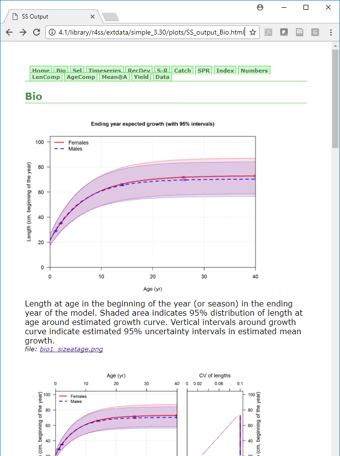
SS_plots() function.Creating select plots
SS_plots() runs slowly due to the large number of plots
created. If only a few plots are of interest, it is more efficient to
plot only the necessary ones. Groups of plots to generate in the call to
SS_plots() can be specified through the plot
argument. For example, if only the plots of Catch were desired,
call:
SS_plots(replist = replist, plot = 7)If only plots of catch and discards were desired, the user could call:
The documentation for the plot argument in the help file
for SS_plots() lists the corresponding numbers for each
group of plots.
It is not uncommon to run into bugs with the plotting functions because of the vast number of model configurations available in SS3 and plots created from them. A strategy with for dealing with a bug is to exclude the set of plots where the bug is occurring as a temporary fix. In the long term, bugs typically get attention fairly quickly from maintainers when reported to the r4ss issue tracker. For example, if there was a bug in the conditional age-at-length fits (plot set 18), exclude the plot:
Scripting Stock Synthesis workflows with r4ss
Using functions in r4ss, a fully scripted workflow for
modifying Stock Synthesis files and running Stock Synthesis models is
possible.
We’ll demonstrate this by creating a new model from a model in the
r4ss package.
# initial model to modify
mod_path <- system.file(file.path("extdata", "simple_small"), package = "r4ss")
# create a new directory to put a new, modified version of the model
new_mod_path <- "simple_new"
Use the r4ss utility function to copy over the model files from
mod_path to new_mod_path:
copy_SS_inputs(dir.old = mod_path, dir.new = new_mod_path)
#> copying files from /home/runner/work/_temp/Library/r4ss/extdata/simple_small to
#> simple_new
#> copying complete
Note that the function populate_multiple_folders() can
be used to copy several folders of Stock Synthesis model inputs.
Read in Stock Synthesis files
Stock Synthesis files can be read in as list objects in R using the
SS_read() function.
inputs <- r4ss::SS_read(dir = new_mod_path)
# can also separately run the functions called by SS_read():
# SS_readstarter(), SS_readdat(), SS_readctl(), SS_readforecast(),
# and SS_readwtatage()
Investigate the model
Each of the input files is read into R as a list which are then
grouped as a larger list. The components of the list should be in the
same order as they appear in the text file. Use names() to
see all the list components:
names(inputs) # see the elements of the big list
#> [1] "dir"   "path"  "dat"   "ctl"   "start" "fore"
names(inputs$start) # see names of the list components of starter file
#>  [1] "sourcefile"             "type"                   "SSversion"
#>  [4] "datfile"                "ctlfile"                "init_values_src"
#>  [7] "run_display_detail"     "detailed_age_structure" "checkup"
#> [10] "parmtrace"              "cumreport"              "prior_like"
#> [13] "soft_bounds"            "N_bootstraps"           "last_estimation_phase"
#> [16] "MCMCburn"               "MCMCthin"               "jitter_fraction"
#> [19] "minyr_sdreport"         "maxyr_sdreport"         "N_STD_yrs"
#> [22] "converge_criterion"     "retro_yr"               "min_age_summary_bio"
#> [25] "depl_basis"             "depl_denom_frac"        "SPR_basis"
#> [28] "F_std_units"            "F_age_range"            "F_std_basis"
#> [31] "MCMC_output_detail"     "ALK_tolerance"          "final"
#> [34] "seed"                   "Compatibility"
Or reference a specific element to see the components. For example, we can look at the mortality and growth parameter section (MG_parms):
inputs$ctl$MG_parms
#>                         LO        HI        INIT       PRIOR PR_SD PR_type
#> NatM_p_1_Fem_GP_1    5e-02  0.150000  0.10000000  0.10000000   0.8       0
#> L_at_Amin_Fem_GP_1   1e+01 45.000000 22.76900000 36.00000000  10.0       0
#> L_at_Amax_Fem_GP_1   4e+01 90.000000 70.31160000 70.00000000  10.0       0
#> VonBert_K_Fem_GP_1   5e-02  0.250000  0.14216500  0.15000000   0.8       0
#> CV_young_Fem_GP_1    5e-02  0.250000  0.10000000  0.10000000   0.8       0
#> CV_old_Fem_GP_1      5e-02  0.250000  0.10000000  0.10000000   0.8       0
#> Wtlen_1_Fem_GP_1    -3e+00  3.000000  0.00000244  0.00000244   0.8       0
#> Wtlen_2_Fem_GP_1    -3e+00  4.000000  3.34694000  3.34694000   0.8       0
#> Mat50%_Fem_GP_1      5e+01 60.000000 55.00000000 55.00000000   0.8       0
#> Mat_slope_Fem_GP_1  -3e+00  3.000000 -0.25000000 -0.25000000   0.8       0
#> Eggs_alpha_Fem_GP_1 -3e+00  3.000000  1.00000000  1.00000000   0.8       0
#> Eggs_beta_Fem_GP_1  -3e+00  3.000000  0.00000000  0.00000000   0.8       0
#> NatM_p_1_Mal_GP_1   -3e+00  3.000000  0.00000000  0.00000000  99.0       0
#> L_at_Amin_Mal_GP_1  -3e+00  3.000000  0.00000000  0.00000000  99.0       0
#> L_at_Amax_Mal_GP_1  -3e+00  3.000000  0.00000000  0.00000000  99.0       0
#> VonBert_K_Mal_GP_1  -3e+00  3.000000  0.00000000  0.00000000  99.0       0
#> CV_young_Mal_GP_1   -3e+00  3.000000  0.00000000  0.00000000  99.0       0
#> CV_old_Mal_GP_1     -3e+00  3.000000  0.00000000  0.00000000  99.0       0
#> Wtlen_1_Mal_GP_1    -3e+00  3.000000  0.00000244  0.00000244   0.8       0
#> Wtlen_2_Mal_GP_1    -3e+00  4.000000  3.34694000  3.34694000   0.8       0
#> CohortGrowDev        1e-01 10.000000  1.00000000  1.00000000   1.0       0
#> FracFemale_GP_1      1e-06  0.999999  0.50000000  0.50000000   0.5       0
#>                     PHASE env_var&link dev_link dev_minyr dev_maxyr dev_PH
#> NatM_p_1_Fem_GP_1      -3            0        0         0         0      0
#> L_at_Amin_Fem_GP_1      2            0        0         0         0      0
#> L_at_Amax_Fem_GP_1      4            0        0         0         0      0
#> VonBert_K_Fem_GP_1      4            0        0         0         0      0
#> CV_young_Fem_GP_1      -3            0        0         0         0      0
#> CV_old_Fem_GP_1        -3            0        0         0         0      0
#> Wtlen_1_Fem_GP_1       -3            0        0         0         0      0
#> Wtlen_2_Fem_GP_1       -3            0        0         0         0      0
#> Mat50%_Fem_GP_1        -3            0        0         0         0      0
#> Mat_slope_Fem_GP_1     -3            0        0         0         0      0
#> Eggs_alpha_Fem_GP_1    -3            0        0         0         0      0
#> Eggs_beta_Fem_GP_1     -3            0        0         0         0      0
#> NatM_p_1_Mal_GP_1      -3            0        0         0         0      0
#> L_at_Amin_Mal_GP_1     -3            0        0         0         0      0
#> L_at_Amax_Mal_GP_1     -3            0        0         0         0      0
#> VonBert_K_Mal_GP_1     -3            0        0         0         0      0
#> CV_young_Mal_GP_1      -3            0        0         0         0      0
#> CV_old_Mal_GP_1        -3            0        0         0         0      0
#> Wtlen_1_Mal_GP_1       -3            0        0         0         0      0
#> Wtlen_2_Mal_GP_1       -3            0        0         0         0      0
#> CohortGrowDev          -1            0        0         0         0      0
#> FracFemale_GP_1       -99            0        0         0         0      0
#>                     Block Block_Fxn
#> NatM_p_1_Fem_GP_1       0         0
#> L_at_Amin_Fem_GP_1      0         0
#> L_at_Amax_Fem_GP_1      0         0
#> VonBert_K_Fem_GP_1      0         0
#> CV_young_Fem_GP_1       0         0
#> CV_old_Fem_GP_1         0         0
#> Wtlen_1_Fem_GP_1        0         0
#> Wtlen_2_Fem_GP_1        0         0
#> Mat50%_Fem_GP_1         0         0
#> Mat_slope_Fem_GP_1      0         0
#> Eggs_alpha_Fem_GP_1     0         0
#> Eggs_beta_Fem_GP_1      0         0
#> NatM_p_1_Mal_GP_1       0         0
#> L_at_Amin_Mal_GP_1      0         0
#> L_at_Amax_Mal_GP_1      0         0
#> VonBert_K_Mal_GP_1      0         0
#> CV_young_Mal_GP_1       0         0
#> CV_old_Mal_GP_1         0         0
#> Wtlen_1_Mal_GP_1        0         0
#> Wtlen_2_Mal_GP_1        0         0
#> CohortGrowDev           0         0
#> FracFemale_GP_1         0         0
Modify the model
You could make basic or large structural changes to your model in R. For example, the initial value of M can be changed:
# view the initial value
inputs$ctl$MG_parms["NatM_p_1_Fem_GP_1", "INIT"]
#> [1] 0.1
# change it to 0.2
inputs$ctl$MG_parms["NatM_p_1_Fem_GP_1", "INIT"] <- 0.2
You can also add new parameters to estimate:
inputs$ctl$Q_options["SURVEY2", "extra_se"] <- 1
inputs$ctl$Q_parms <- SS_add_parameter_line(par_df = inputs$ctl$Q_parms,
                                            row_to_copy = 2,
                                            row_before = "base_SURVEY2",
                                            newval_df = data.frame(rowname = "extraSD_survey2",
                                                                   INIT = 0.05,
                                                                   PHASE = 4))
When making large structural changes, additional elements may need to
be added that were NULL before. To find out the names in the r4ss list
object, it may be necessary to make changes directly to the input files
and then read it in again to R, or to look at the source code for the
names of the list elements. For example, the source code for
SS_readctl() when using a SS3.30 file is located at https://github.com/r4ss/r4ss/blob/main/R/SS_readctl_3.30.R.
Settings in other files can also be modified. For example, the biomass target can be modified in the forecast file
inputs$fore$Btarget
#> [1] 0.4
inputs$fore$Btarget <- 0.45
inputs$fore$Btarget
#> [1] 0.45
Write out the modified models
The SS_write() function can be used to write out the
modified stock synthesis input R objects into input files:
r4ss::SS_write(inputs, dir = new_mod_path, overwrite = TRUE)If you make changes to the input model files that render the file
unparsable by Stock Synthesis, the SS_write() function may
throw an error (and hopefully provide an informative message about why).
However, it is possible that an invalid Stock Synthesis model file could
be written, so the true test is whether or not it is possible to run
Stock Synthesis with the modified model files.
If you need help troubleshooting SS_read() or
SS_write() and the associated functions for each model
file, or would like to report a bug, please post an issue in the r4ss
repository.
Download the Stock Synthesis executable from GitHub
The latest release of the Stock Synthesis executable or other releases found by entering a character string of a version tag (list of tags is available here) can be downloaded from the Stock Synthesis GitHub page using the function:
# Default with no version downloads the latest release
r4ss::get_ss3_exe()

# Download the latest release to a specific directory
r4ss::get_ss3_exe(dir = new_mod_path)

# Adding a character string for a specific version using the GitHub tag
r4ss::get_ss3_exe(dir = new_mod_path, version = "v3.30.18")
You can also use the function without a specified directory which will download the executable to your working directory. This function downloads the correct executable according to information it gets about your operating system.
Run the modified model
The model can now be run with Stock Synthesis. The call to do this
depends on where the Stock Synthesis executable is on your computer. If
the Stock Synthesis executable is in the same folder as the model that
will be run, run() can be used. Assuming the stock
synthesis executable is called ss.exe:
r4ss::run(dir = new_mod_path, skipfinished = FALSE)Note this is similar to resetting the working directory and running
the model with system() or shell(), but deals
with differences among operating systems automatically. Another
advantage of run() is that there is no need to change the
working directory.
If the executable in a different folder than the model, specify
either the absolute or relative path to the executable. Note that
executables for v3.30.22.1 and after are named ss3.exe, ss3_linux, and
ss3_osx unless you download the executables using
get_ss3_exe() which gives them the names ss3.exe (for
windows) and ss3 (for linux/osx) regardless of the version.
# use the absolute exe path in the call on a Windows computer.
run(dir = new_mod_path, exe = "c:/SS/SSv3.30.19.01_Apr15/ss.exe")
# use the absolute exe path in the call on linux.
run(dir = new_mod_path, exe = "~/SS/SSv3.30.19.01_Apr15/ss_linux")
Finally, if the stock synthesis executable is in your PATH, then
run() should find it automatically.
Investigate the model run
As previously, SS_output() and
SS_plots() can be used to investigate the model
results.
Should I script my whole Stock Synthesis workflow?
Scripting using r4ss functions is one way of developing a reproducible and coherent Stock Synthesis development workflow. However, there are many ways that Stock Synthesis models could be run and modified. What is most important is that you find a workflow that works for you and that you are able to document changes being made to a model. Version control (such as git) is another tool that may help document changes to models.
Functions for common stock assessment tasks
While stock assessment processes differ among regions, some modeling
workflows and diagnostics are commonly used. Within r4ss, there are
functions to perform a retrospective (retro()), jitter the
starting values and reoptimize the stock assessment model a number of
times to check for local minima (jitter()) and tuning
composition data (tune_comps()).
Additional model diagnostics for Stock Synthesis models are available as part of the ss3diags package.
Running retrospectives
A retrospective analysis removes a certain number of years of the model data and recalculates the fit. This is typically done several times and the results are used to look for retrospective patterns (i.e., non-random deviations in estimated parameters or derived quantities as years of data are removed). If the model results change drastically and non-randomly as data is removed, this is less support for the model. For more on the theory and details behind retrospective analyses, see Hurtado-Ferro et al. 2015 and Legault 2020.
The function retro() can be used to run retrospective
analyses starting from an existing Stock Synthesis model. Note that it
is safest to create a copy of your original Stock Synthesis model that
the retrospective is run on, just in case there are problems with the
run. For example, a five year retrospective could be done:
# create a temporary path for the retrospective analyses to run and download the
# ss3 exe
old_mod_path <- system.file(file.path("extdata", "simple_small"), package = "r4ss")
new_mod_path <- tempdir()
all_files <- list.files(old_mod_path, full.names = TRUE)
file.copy(from = all_files, to = new_mod_path)
get_ss3_exe(dir = new_mod_path)
# run the retrospective analyses
retro(
  dir = new_mod_path, # wherever the model files are
  oldsubdir = "", # subfolder within dir
  newsubdir = "retrospectives", # new place to store retro runs within dir
  years = 0:-5, # years relative to ending year of model
  exe = "ss3"
)
After running this retrospective, six new folders would be created within a new “retrospectives” directory, where each folder would contain a different run of the retrospective (removing 0 to 5 years of data).
After the retrospective models have run, the results can be used as a diagnostic:
# load the 6 models
retroModels <- SSgetoutput(dirvec = file.path(
  new_mod_path, "retrospectives",
  paste("retro", 0:-5, sep = "")
))
# summarize the model results
retroSummary <- SSsummarize(retroModels)
# create a vector of the ending year of the retrospectives
endyrvec <- retroSummary[["endyrs"]] + 0:-5
# make plots comparing the 6 models
# showing 2 out of the 19 plots done by SSplotComparisons
SSplotComparisons(retroSummary,
  endyrvec = endyrvec,
  legendlabels = paste("Data", 0:-5, "years"),
  subplot = 2, # only show one plot in vignette
  print = TRUE, # send plots to PNG file
  plot = FALSE, # don't plot to default graphics device
  plotdir = new_mod_path
)
knitr::include_graphics(file.path(new_mod_path, "compare2_spawnbio_uncertainty.png"))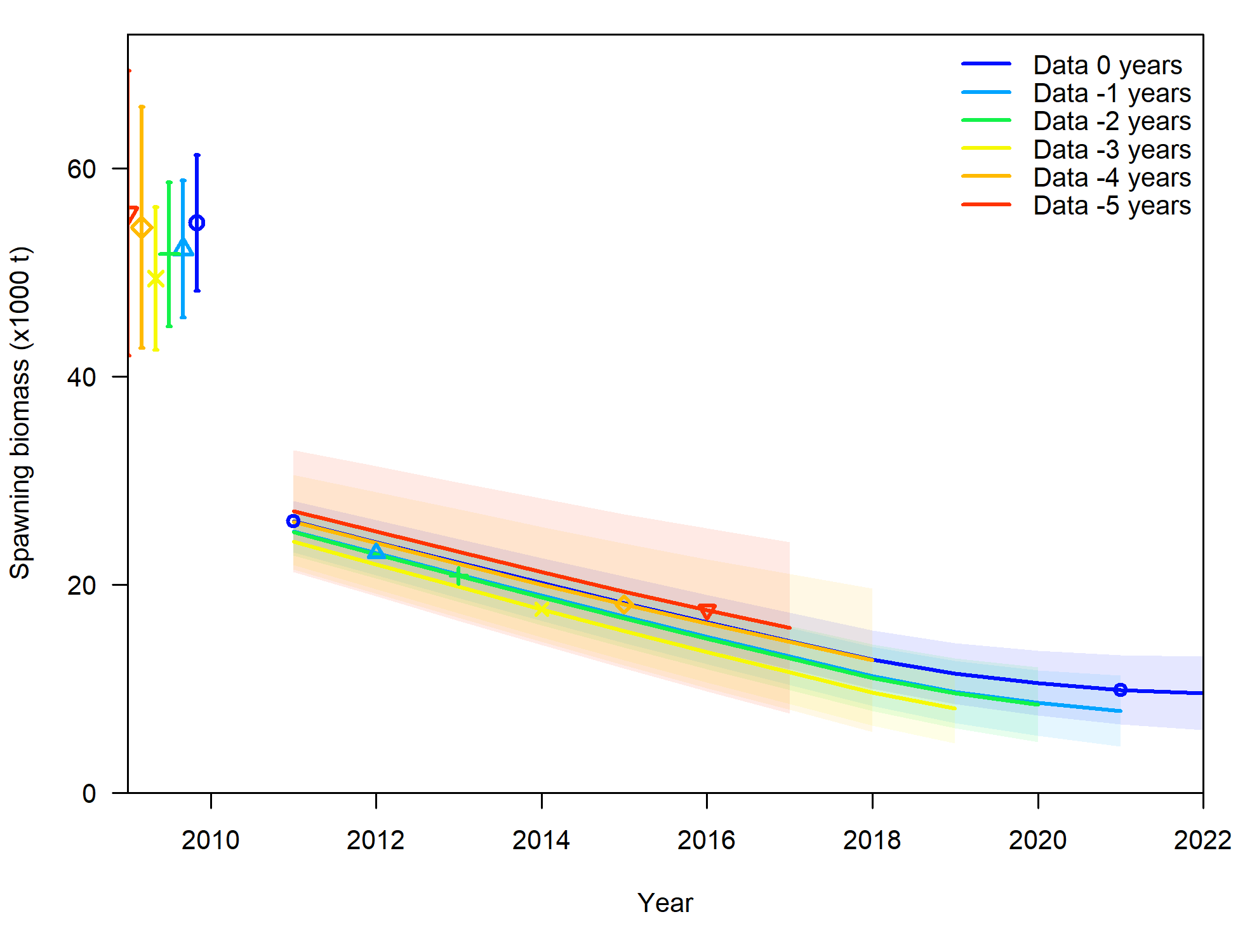
SSplotComparisons() function.
# calculate Mohn's rho, a diagnostic value
rho_output <- SSmohnsrho(
  summaryoutput = retroSummary,
  endyrvec = endyrvec,
  startyr = retroSummary[["endyrs"]] - 5,
  verbose = FALSE
)
Jittering
Another commonly used diagnostic with Stock Synthesis models is
“jittering”. Model initial values are changed randomly (by some fraction
in a transformed parameter space) and the model is reoptimized. The
jitter() function performs this routine for the number of
times specified by the user. For a stock Synthesis model in a folder
called jitter_dir jittering starting values can be run 100
times (note this could take a while as they will be run in
sequence):
# define a new directory
jitter_dir <- file.path(mod_path, "jitter")
# copy over the stock synthesis model files to the new directory
copy_SS_inputs(dir.old = mod_path, dir.new = jitter_dir)
# run the jitters
jitter_loglike <- jitter(
  dir = jitter_dir,
  Njitter = 100,
  jitter_fraction = 0.1 # a typically used jitter fraction
)
The output from jitter() is saved in
jitter_loglike, which is a table of the different negative
log likelihoods produced from jittering. If there are any negative log
likelihoods smaller than the original model’s log likelihood, this
indicates that the original model’s log likelihood is a local minimum
and not the global minimum. On the other hand, if there are no log
likelihoods lower than the original model’s log likelihood, then this is
evidence (but not proof) that the original model’s negative log
likelihood could be the global minimum.
Jittering starting values can also provide evidence about the sensitivity of the model to starting values. If many different likelihood values are arrived at during the jitter analysis, then the model is sensitive to starting values. However, if many of the models converge to the same negative log likelihood value, this indicates the model is less sensitive to starting values.
Tuning composition data
Three different routines are available to tune (or weight) composition data in Stock Synthesis. The McAllister-Ianelli (MI) and Francis tuning methods are iterative reweighting routines, while the Dirichlet-multinomial (DM) option incorporates weighting parameters directly in the original model.
Because tuning is commonly used with Stock Synthesis models, and
users may be interested in exploring the same model, but using different
tuning methods, tune_comps() can start from the same model
and transform it into different tuning methods.
As an example, we will illustrate how to run Francis tuning on an example Stock Synthesis model built into the r4ss package. First, we make a copy of the model to avoid changing the original model files
# define a new directory in a temporary location
mod_path <- file.path(tempdir(), "simple_mod")
# Path to simple model in r4ss and copy files to mod_path
example_path <- system.file("extdata", "simple_small", package = "r4ss")
# copy model input files
copy_SS_inputs(dir.old = example_path, dir.new = mod_path)
#> copying files from /home/runner/work/_temp/Library/r4ss/extdata/simple_small to
#> /tmp/Rtmp7SbK75/simple_mod
#> copying complete
# copy over the Report file to provide information about the last run
file.copy(
  from = file.path(example_path, "Report.sso"),
  to = file.path(mod_path, "Report.sso")
)
#> [1] TRUE
# copy comp report file  to provide information about the last run of this model
file.copy(
  from = file.path(example_path, "CompReport.sso"),
  to = file.path(mod_path, "CompReport.sso")
)
#> [1] TRUE
The following call to tune_comps() runs Francis
weighting for 1 iteration and allows upweighting. Assume that an
executable called “ss or ss.exe” is available in the mod_path
folder.
tune_info <- tune_comps(
  option = "Francis",
  niters_tuning = 1,
  dir = mod_path,
  allow_up_tuning = TRUE,
  verbose = FALSE
)
# see the tuning table, and the weights applied to the model.
tune_info
Now, suppose we wanted to run the same model, but using
Dirichlet-multinomial parameters to weight. The model can be copied over
to a new folder, then the tune_comps() function could be
used to add Dirichlet-multinomial parameters (1 for each fleet with
composition data and for each type of composition data) and re-run the
model.
# create additional temporary directory
mod_path_dm <- file.path(tempdir(), "simple_mod_dm")
# copy model files
copy_SS_inputs(dir.old = mod_path, dir.new = mod_path_dm, copy_exe = TRUE)
# copy over the Report file to provide information about the last run
file.copy(
  from = file.path(mod_path, "Report.sso"),
  to = file.path(mod_path_dm, "Report.sso")
)
# copy comp report file  to provide information about the last run of this model
file.copy(
  from = file.path(mod_path, "CompReport.sso"),
  to = file.path(mod_path_dm, "CompReport.sso")
)
# Add Dirichlet-multinomial parameters and rerun. The function will
# automatically remove the MI weighting and add in the DM parameters.
DM_parm_info <- tune_comps(
  option = "DM",
  niters_tuning = 1, # must be 1 or greater to run, through DM is not iterative
  dir = mod_path_dm
)
# see the DM parameter estimates
DM_parm_info[["tuning_table_list"]]
There are many options in the tune_comps() function;
please see the documentation (?tune_comps in the R console)
for more details and examples.